

Compare the distribution of individual packing times alongside their mean. Two observed groups can have the same average and total work yet very different slow-order tails. An explicitly defined percentile helps describe that difference without turning a tiny timing exercise into a production promise.

Preserve the complete clock and order definition
Use the same observable start and finish, included tasks and units for every duration being compared. State the product configuration, operator conditions and interruptions. The packing-trial record establishes that observation scope; the distribution summary comes afterwards.
Do not silently delete a long observation because it contains a retrieval, unclear instruction or rework event. Retain the raw duration and its explanation. If you also calculate a summary excluding a defined event, name the altered scope and show both results.
This article asks which observations make the tail long. It does not divide a shift by an assumed cycle time, decide staffing or prove that a changed box caused the difference.
Compare two invented five-order groups
Assume the following durations cover the same defined packing task. They are fictional seconds, already sorted from shortest to longest, not observed Packrivo or customer performance.
Scroll horizontally if columns extend beyond the view.
| Summary field | Group A | Group B |
|---|---|---|
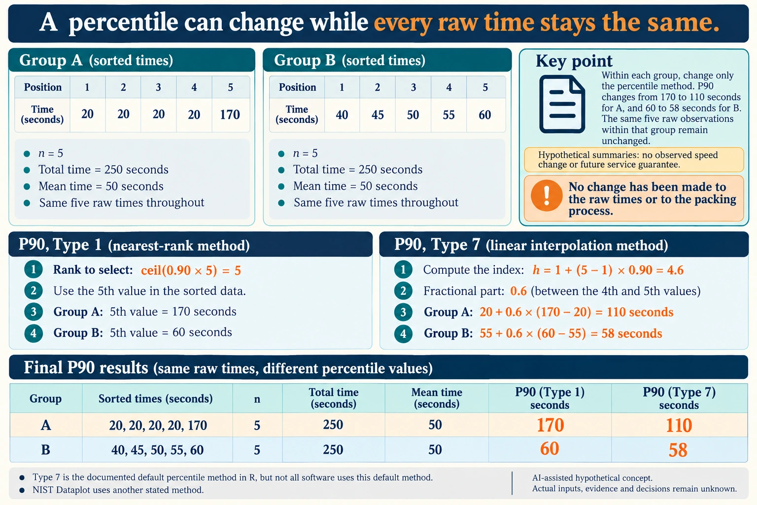
| Sorted durations, seconds | 20, 20, 20, 20, 170 | 40, 45, 50, 55, 60 |
| Number of observations | 5 | 5 |
| Total observed work | 250 seconds | 250 seconds |
| Arithmetic mean | 50 seconds | 50 seconds |
| Median under the method below | 20 seconds | 50 seconds |
| Observed 90th percentile | 170 seconds | 60 seconds |
| Maximum observed duration | 170 seconds | 60 seconds |
The identical means do not reveal that Group A contains four short durations and one much longer duration. Group B’s observations are more closely grouped. Calling both “50-second packing” would lose that distinction.
State exactly how the percentile is calculated
For this worksheet, use an empirical nearest-rank method: sort n observations in ascending order; multiply n by the requested percentile expressed as a fraction; round the rank up to the next integer; take the observation at that rank. Ranks start at one.
For the 90th percentile with five observations, the rank is the ceiling of 0.90 x 5 = 4.5, which is five. The fifth values are 170 and 60 seconds. For the median, the rank is the ceiling of 0.50 x 5 = 2.5, which is three, giving 20 and 50 seconds.
This explicit method matters. NIST’s Dataplot documentation describes several percentile calculations and notes that their results can differ, particularly for small samples. Its default interpolated calculation is not the nearest-rank rule chosen here. Record the software method if a spreadsheet supplies the result. The official R quantile reference describes a type-one inverse empirical method consistent with selecting these observed ranks; this is not its default calculation.
Interpret the observed tail without promising a service level
With only five rows, the nearest-rank 95th percentile also uses rank five. It adds no extra information beyond the maximum in this example. These five invented observations cannot establish that 95% of future orders will finish within that duration.
Likewise, Group A’s one observation above sixty seconds and Group B’s zero describe these lists only. They are not reliable estimates of future exception frequency. Larger, appropriately collected evidence and the actual order mix are needed before making operational commitments.
Trace the long observation back to its task record. A product type, message-matching step or replenishment event might deserve a separate group or investigation. The duration alone does not identify the cause or justify removing the event.
Return a timing summary containing the raw durations, sample count, clock definition, mean, median, chosen percentile method and observed maximum. That gives the packing owner a specific tail to investigate while preserving the original observations.
Source scope: NIST’s percentile documentation was checked on 15 October 2026. It supports method transparency and percentile concepts, not a packaging speed, sample-size guarantee or promised throughput.
Hold the raw times fixed when comparing percentile methods
Use the same five fictional durations already listed above. Change only the summary method. Nearest-rank type one selects rank ceiling(0.90 × 5) = 5, so P90 remains 170 seconds for A and 60 seconds for B. These are not new packing observations.
Scroll horizontally if columns extend beyond the view.
| Hypothetical scenario | Item or operation | Planning relationship | Assumed input or calculation |
|---|---|---|---|
| QUANTILE35 | TYPE7_ONE_BASED_INDEX | calculated from | 1+(O_N-1)*O_P90; 4.6 index |
| QUANTILE35 | LOWER_ORDER_STATISTIC_INDEX | calculated from | floor(H7); 4 index |
| QUANTILE35 | NEXT_ORDER_STATISTIC_INDEX | calculated from | LOWER_INDEX+1; 5 index |
| QUANTILE35 | INTERPOLATION_FRACTION | calculated from | H7-LOWER_INDEX; 0.6 fraction |
| QUANTILE35 | A_P90 | calculated from | O_A4+FRACTION*(O_A5-O_A4); 110 seconds |
| QUANTILE35 | B_P90 | calculated from | O_B4+FRACTION*(O_B5-O_B4); 58 seconds |
For type seven, the one-based index is h = 1 + (5 − 1) × 0.90 = 4.6. Interpolate six-tenths of the distance between the fourth and fifth observations. A gives 20 + 0.6 × (170 − 20) = 110 seconds. B gives 55 + 0.6 × (60 − 55) = 58 seconds. Each group’s raw list, count, total and mean remain unchanged.
A dashboard could therefore display a lower P90 after a method change even though no packing work became faster. Keep the percentile definition with the exported raw durations and compare like with like before interpreting a reported improvement. The CSV links each selected fourth or fifth value to its original sample position.
The public R reference documents type seven as its default and type one separately. The reviewed page is R-devel documentation, not evidence of a particular installed or stable R version; NIST Dataplot’s stated default is another method. No software execution or preferred method is claimed here. Neither interpolation nor the earlier nearest-rank result establishes a future service percentile from five invented rows.
Download the packing time percentile method type1 type7 comparison record (.csv). It includes the original table fields and scenarios alongside the added relationships. HYPOTHETICAL rows are editorial examples or required review scopes, not actual records. Actual quantity, configuration, component and file identities, materials, process, specification, copy, method, condition, observation, owner, decision, evidence and dates are blank. ACTUAL_BLANK is a separate empty starting row; enter permitted project evidence before using an actual record. A blank means unknown.
Use the Record a Packing Trial Without Promising a Universal Speed for its separate question.
Source scope checked 17 October 2026: The current R-devel stats quantile page documents type one and type seven, with type seven the R default; no installed R execution is claimed. NIST Dataplot’s method discussion is distinct. Five invented times do not establish a future percentile guarantee. The added configurations and calculations are hypothetical, with actual evidence and decisions pending.
What this changes in a packaging enquiry
If slow packing orders influence a packaging change, identify the physical task behind those observations before asking for a different delivered state or structure. Use the same order definition in the comparison. The illustrative percentiles do not establish supplier performance or prove that new packaging will remove the delays.
Discuss this packaging specification with Packrivo. We coordinate independent suppliers. MOQ: 500 pieces per product/design; illustrative quantities are not production offers. Confirm materials, samples, price and timing for your project.